
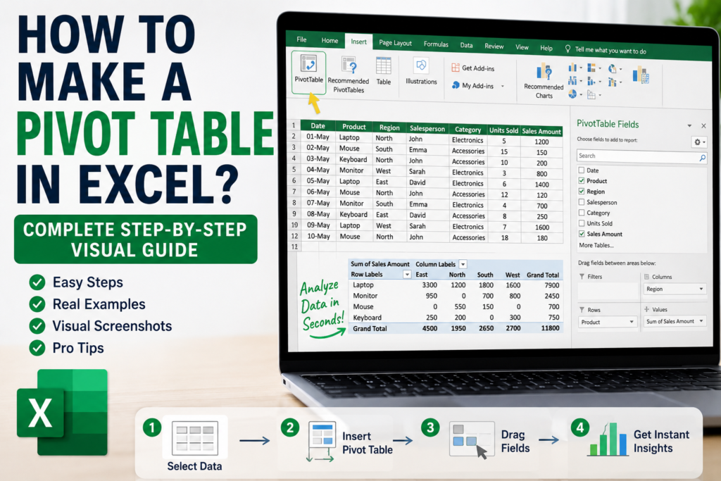
How to Make a Pivot Table in Excel?
Imagine your boss sends you an Excel file containing 5,000 rows of sales data and asks:
“Can you tell me which product generated the highest sales and which region performed best?”
Your first thought might be:
“Do I need complicated formulas?”
Many people start manually filtering data, writing formulas, and scrolling endlessly through spreadsheets.
But experienced Excel users usually solve this problem in less than a minute.
They use one of Excel’s most powerful hidden tools:
Pivot Tables
A Pivot Table can summarize thousands of rows instantly without writing complex formulas.
In this guide you’ll learn exactly how to create a Pivot Table step by step using real examples.
What Is a Pivot Table in Excel?
A Pivot Table is an Excel feature that helps organize, summarize, and analyze large amounts of data quickly.
Instead of manually calculating totals, Excel automatically groups and summarizes information.
You can instantly answer questions like:
- Which product sold the most?
- Which region generated highest revenue?
- Who is the best salesperson?
- What is total monthly sales?
Why Use Pivot Tables?
Pivot Tables save massive amounts of time.
Benefits include:
- Analyze thousands of rows instantly
- No complicated formulas required
- Create reports quickly
- Identify trends easily
- Build dashboards faster
Many professionals use Pivot Tables daily because they reduce manual work significantly.
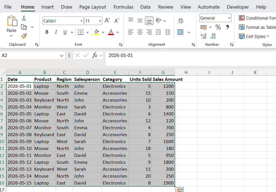
Example Dataset We Will Use
Let’s assume we have sales data:
| Date | Product | Region | Sales |
|---|---|---|---|
| 01-May | Laptop | North | $1200 |
| 02-May | Monitor | West | $800 |
| 03-May | Mouse | East | $150 |
Step 1: Select Your Data
Highlight all rows and columns containing data.
Do not select empty rows because they may create issues later.
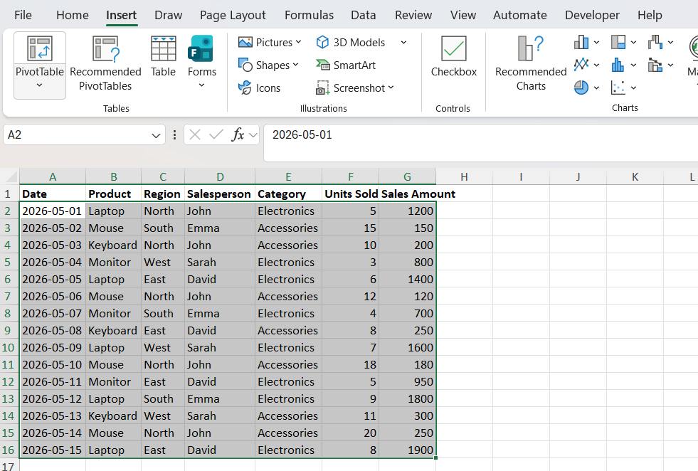
How to Make a Pivot Table in Excel
Step 2: Click Insert → Pivot Table
Go to:
Insert → Pivot Table
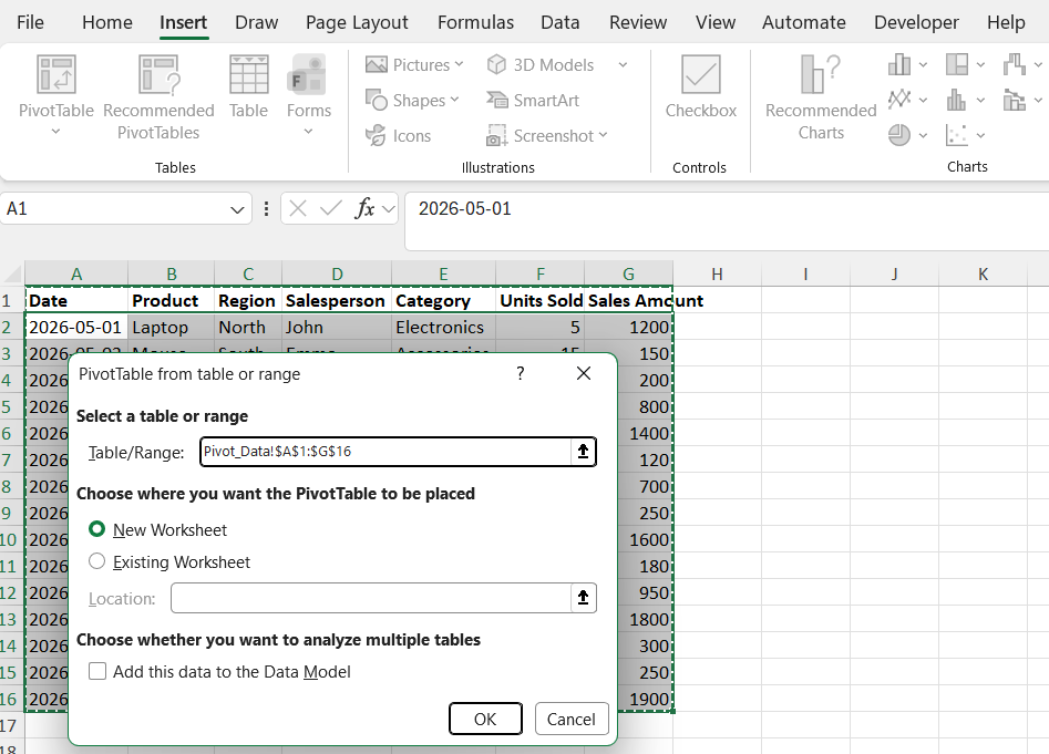
Step 3: Choose Data Range
Excel automatically detects your selected range.
You will see a dialog box asking:
- Select table/range
- Choose where Pivot Table should appear
Select:
New Worksheet
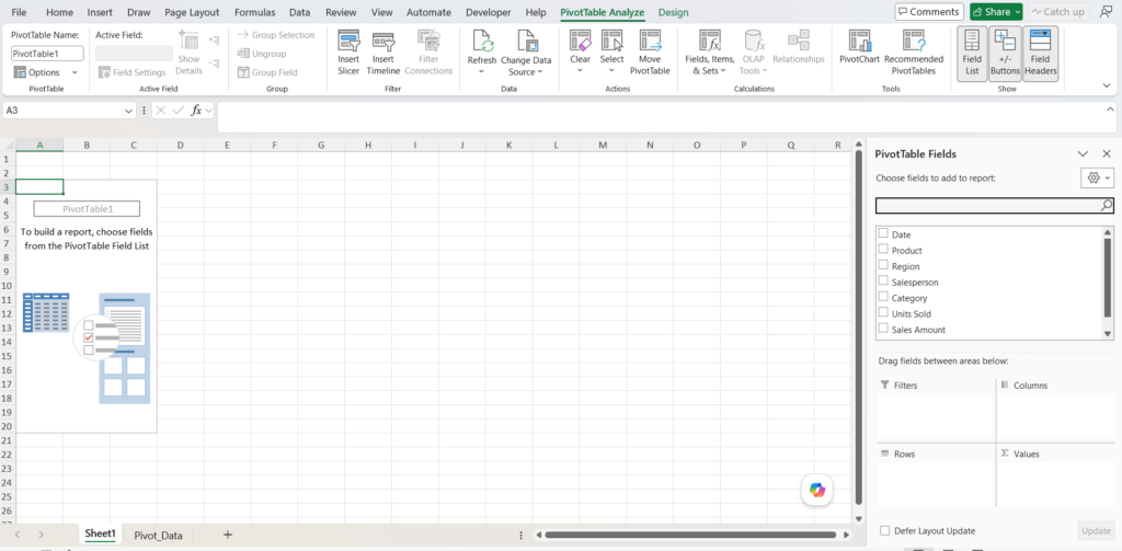
Step 4: Build Your First Pivot Table
Now the Pivot Table Fields panel appears.
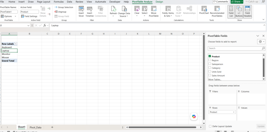
Drag fields like this:
- Product → Rows
- Sales → Values
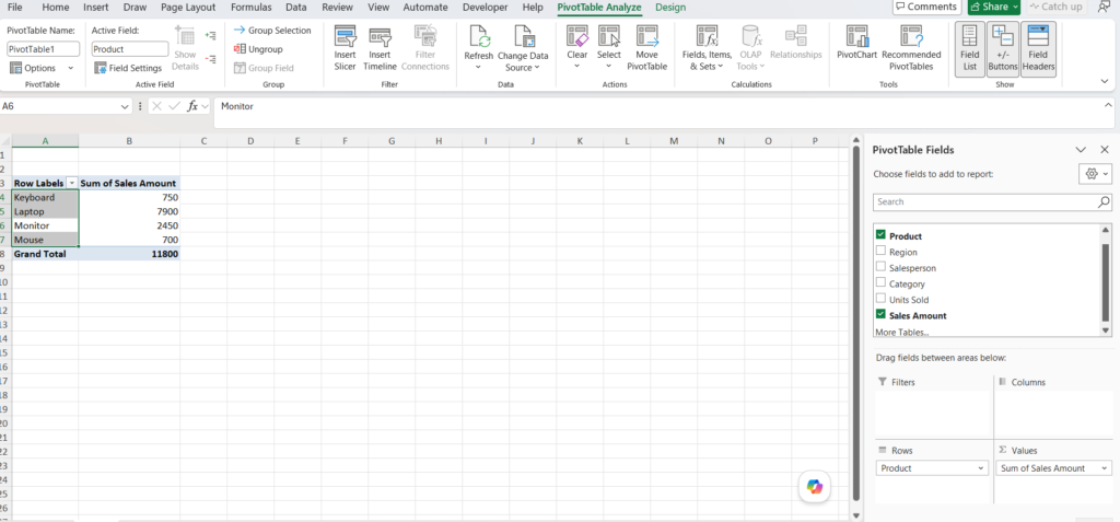
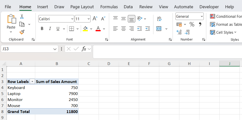
Excel instantly creates a summarized report.
What Just Happened?
Excel automatically calculated total sales for every product.
Without formulas.
Without filtering.
Without manual calculations.
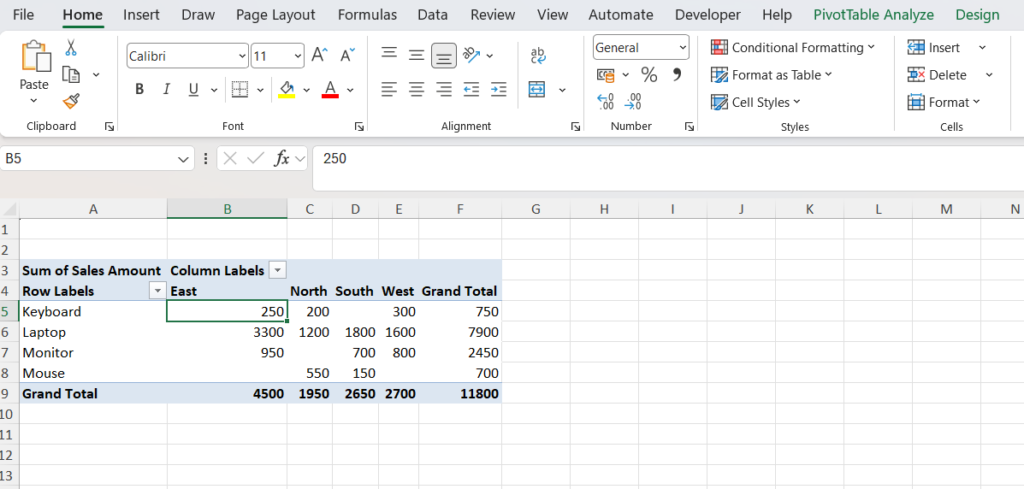
Advanced Example
Let’s make the report smarter.
Drag:
- Region → Columns
- Sales → Values
- Product → Rows
Now Excel creates a report showing:
- Sales by region
- Sales by product
- Total sales
Common Pivot Table Mistakes
- Including blank rows
- Selecting incomplete data
- Not refreshing Pivot Tables
- Using inconsistent data formats
If your source data changes, right-click Pivot Table and select Refresh.
Related Articles
Frequently Asked Questions
What is a Pivot Table?
A Pivot Table summarizes large amounts of Excel data quickly.
Can beginners use Pivot Tables?
Yes. Pivot Tables are beginner-friendly.
Do Pivot Tables update automatically?
No. You need to click Refresh after changing source data.


Pingback: Top Pivot Table Interview Questions and Answers (2026 Guide) - Excel AI Tools and SEO Guides
Pingback: Excel Arrow Keys Not Moving Cells? Here's the Quick Fix (Step-by-Step Guide 2026) - Excel AI Tools and SEO Guides